Day 19 - Sinusoids and Phasors Cont.

Topics Discussed

On day 19 of the ENGR 44 course, we had further discussion of sinusoids and phasors. Additionally, we were introduced to the concept of impedance in different elements of a circuit such as capacitors, inductors, and resistors. We were also introduced to the concept of admittance which is essentially the inverse of impedance. We did several practice problems with these ideas in mind. (Fig. 1) We also discussed the concept of leading and lagging in terms of voltage and current, and how different elements within the circuit can experience this. (Fig. 2)

Fig. 1

Fig. 2

Impedance Lab

In lab, we planned to investigate the effects of a sinusoidal voltage at a set frequency on a capacitor, resistor, and inductor in three separate circuits. We wanted to use frequency at 1kHz, 5kHz, and 10kHz. We then converted these to omega and made some calculations in reference to the responses we should get. (Fig. 3)

Fig. 3

Once the calculations were complete, we then proceeded to create each circuit. (Fig. 4,5,6) 

Fig. 4 - Inductor

Fig. 5 - Capacitor

Fig. 6 - Resistor

We then applied the three different frequencies to each circuit and observed the effects on the voltage gain across each. (Fig. 7-15)

Fig. 7 - Inductor @ 6280 Hz

Fig. 8 - Inductor @ 31 kHz

Fig. 9 - Inductor @ 62 kHz

Fig. 10 - Capacitor @ 6283 Hz

Fig. 11 - Capacitor @ 31 kHz

Fig. 12 - Capacitor @ 62 kHz

Fig. 13 - Resistor @ 6283 Hz

Fig. 14 - Resistor @ 31 kHz

Fig. 15 - Resistor @ 62 kHz

Summary

Upon completion of the lab, we were able to successfully view the effects of applying these different frequency voltages to these separate elements in each circuit.

Day 18 - Sinusoids and Phasors

Topics Discussed

On day 18 of the ENGR 44 course, we were introduced to the topics of sinusoids and phasors. Sinusoids are signals that vary according to an alternating sine or cosine function. We did several practice problems with these concepts. (Fig. 1) We also discussed using phasors which are phase shifts within these sinusoids. We practiced several methods used to add, subtract, multiply, and divide these phasors, including how to convert them from polar to rectangular coordinates and vice-versa.

Fig. 1

Passive RL Circuit Response Lab

In lab we planned to make an RL circuit and analyze the effects on said circuit when applying a sinusoidal voltage function. Using the phase shift within our calculations, we were able to find theoretical amplitude gains that were given by a formula within the lab manual. (Fig. 2)

Fig. 2

Once we had our theoretical values, we then proceeded to create the circuit and analyzed the phase shift and gains and found that we were relatively close to our theoretical values. (Fig. 3)

Fig. 3

Summary

Upon completion of the lab, we were able to successfully analyze an RL circuit that had an alternating voltage applied to it. We were able to find the gain and phase shift across the inductor and resistor. Since AC circuits are the most common circuits we find based off of the alternating nature of circuits in our day-to-day lives, being able to properly investigate the effects on certain elements in the circuit becomes extremely useful. 

Day 17 - Second Order Circuits Cont.

Topics Discussed

On day 17 of the ENGR 44 course, we further discussed the topic of second order circuits and how to analyze different elements within the circuit. We were introduced to new techniques and again did some practice problems. (Fig. 1)

Fig. 1

RLC Circuit Response Lab

In lab, we planned to investigate how another version of an RLC circuit would respond when an alternating voltage was applied to it. We calculated values for the theoretical natural frequency and oscillation frequencies. (Fig. 2) Once these values were found, we built the circuit. (Fig. 3)

Fig. 2

Fig. 3

Summary
Despite some alteration to this circuit as opposed to previous RLC circuits, we were able to use the same methods to find several of the characteristics of the circuit, such as natural frequency, oscillation frequency, and whether the system could be considered critically, over-, or under-damped. 

Day 16 - 2nd Order Circuits

Topics Discussed

On day 16 of the ENGR 44 course, we discussed 2nd order circuits. We discussed heavily the importance of understanding the initial conditions of RLC circuits and how they can be used to determine the behavior of these circuits. We also discussed source-free circuits and the tools and equations that can be used to uncover how these circuits behaved. We did a multitude of problems focusing on whether a system was damped, over damped, or critically damped. (Fig. 1) Additionally, we did some practice with source free circuits with granted initial conditions. (Fig. 2). We further derived some expression that we would commonly use throughout these types of problem. (Fig. 3)

Fig. 1

Fig. 2

Fig. 3

Series RLC Circuit Step Response Lab

In lab today, we investigated the voltage response of an RLC circuit when inputting a square wave voltage. We intended to find the alpha, tau, natural frequency, damping ratio, and other various pieces of information relative to our circuit. We first drew up a schematic for the circuit and found the according pieces of information that would be used as our theoretical values. (Fig. 4) Once this was complete, we proceeded to create the actual circuit. (Fig. 5) 

Fig. 4

Fig. 5

Upon completion, we ran the circuit and proceed to analyze the voltage response. (Fig. 6) We drew up several experimental values and compared them to what was originally expected.

Fig. 6

Summary

Upon completion of the lab, we were drawn to one value in particular that stuck out, which was our measured/experimentally calculated tau. We had originally expected a much shorter period for a single oscillation but found one to be relatively 1/4 of a second. This may have been accounted for in the additional resistance of the circuit, which would have increased our alpha and thus decreased our tau. 

Day 15 - First Order Circuits Cont.

Topics Discussed

On day 15 of the ENGR 44 course, we further discussed first order circuits. We discussed unit step functions and how they can apply to RLC circuits and likewise. We also did a multitude of practice problems concerned with finding the voltages across different elements in terms of these unit step functions. (Fig. 1) We also derivated in class the voltage of an RC circuit. (Fig. 2) We also predicted the voltage in an RC circuit given different input voltages of various shapes.. (Fig. 3)

Fig. 1

Fig. 2

Fig. 3

Inverting Differentiator Lab

In the inverting differentiator lab, we sought to make a classic inverting differentiator using a capacitor, resistor, and op-amp. We calculated a multitude of theoretical gains when inputting different frequencies into the circuit, and we planned to use these frequencies and find an experimental gain for comparison. Sample calculations can be seen in Fig. 4.

Fig. 4

Once we had our experimental values accounted for, we proceeded to create the circuit. (Fig. 5) Upon completion of the circuit, we hooked up our circuit to our analog discovery device and began taking measurement. We tried different signals at 100 Hz, 230 Hz, and 500 Hz. (Fig. 6, Fig. 7, Fig. 8).

Fig. 5

Fig. 6 - 100 Hz

Fig. 7 - 230 Hz

Fig. 8 - 500 Hz

Once our measurements were taken, we created a table to document our theoretical versus experimental gains. We found that our highest percent error was below 8%. (Fig. 9)

Fig. 9

Summary

In today's lab, we were able to verify the theoretical gains and our perceived relationship of input to output voltage of an inverting differentiator. With a percent error of less than 8%, our predicted gains at different frequencies held true. 

Day 14 - First Order Circuits

Topics Discussed

On day 14 of the ENGR 44 course, we were introduced to first order circuits. These circuits are known as either RL or RC circuits (resistor-inductor or resistor-capacitor, respectively). These circuits contain the passive elements such as resistors, capacitors, and inductors, and one active element being the operational amplifier. We discussed several relationships to the voltage or current through a capacitor or inductor, and how we can essentially model the behavior of these elements in such a circuit. We did example problems that included deriving an equation for the voltage across a capacitor and the time constant tau associated with the equation. (Fig. 1, Fig. 2, & Fig. 3) "The time constant of a circuit is essentially the amount of time required for the response to decay by a factor of 1/e." (Mason- Lecture Notes). For capacitors, it is RC and for inductors it is L/R. We also did work with inductors in example problems and modeled the current through it as a function of time. (Fig. 4)

Fig. 1 

Fig. 2

Fig. 3

Fig. 4

Passive RC Circuit Natural Response Lab

In lab, we sought to create a simple RC circuit and observe its natural response when an input voltage is applied. We would first model the circuit in a schematic and estimate the time constant. This would allow us to create a theoretical value for how long the capacitor would take to discharge. We would use the oscilloscope trigger to determine the response of the capacitor when voltage was disconnected, or when a square wave was applied. We first created the schematic and made our predictions. (Fig. 6) Once this was done, we created the actual circuit. (Fig. 7)

Fig. 6

Fig. 7

Upon creation of the circuit, we hooked up our analog discovery device and set up an oscilloscope window to observe the specific changes occurring within the capacitor. Perhaps the most difficult aspect of this lab was properly setting up the trigger, which would ultimately determine whether or not we could get a good reading from the oscilloscope window. We found our reading. (Fig. 8) We found that our value for Tau compared to our calculated value was very close and exhibited a percent error of roughly 10%. (Fig. 9)

Fig. 8

Fig. 9

Passive RL Circuit Natural Response Lab

Although we did not necessarily get a chance to complete this in class, we recreated a similar circuit to the when mentioned above, only this time we used an inductor. We again created the schematic and made predictions for the general equaion describing the current as a function of time (Fig. 10) Prior to leaving class, we quickly assembled the circuit and ran a quick trial to observe the response of the inductor. (Fig. 11) 

Fig. 10

Fig. 11

Summary

We were able to successfully assemble and verify our models for the natural response of an RC and RL circuit today in lab. Considering our only measured and recorded trials, the RC circuit exhibited only a rough 10% error in tau when compared to our calculated value. By understanding the process by which these circuits operate, we will be able to create more complex and versatile circuits in the future.

Day 13 - Capacitors and Inductors

Topics Discussed

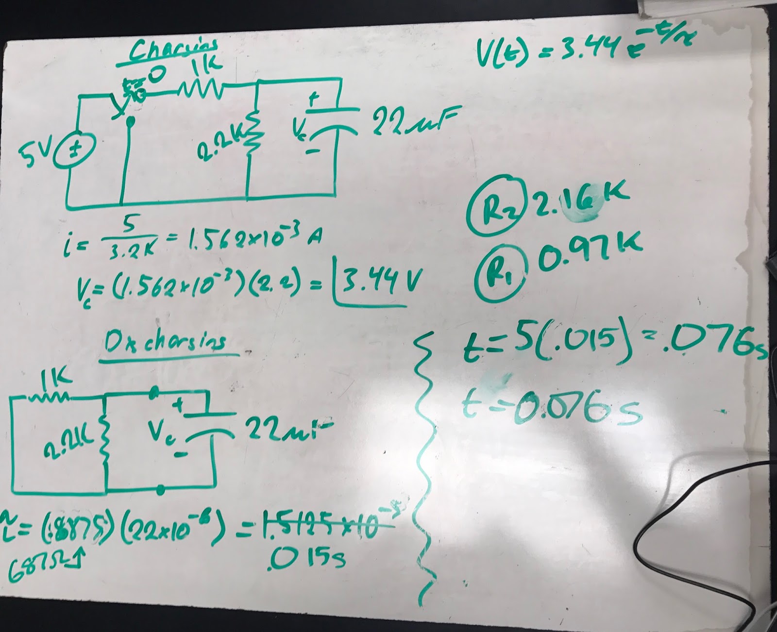
On day 13 of the ENGR 44 course, we were introduced to the basics of capacitors and inductors. We discussed the fundamental workings of capacitors first, noting that they work as a short before being charged and an open after being charged. We also viewed what happens when a capacitor is not aligned correctly relative to the direction of current flowing through it. (Video 1) No one wants to lose their fingers, so this demonstration was both important and entertaining, so we did it twice. We discussed how resistors must accommodate capacitors to prevent sparks from happening in circuits, and we did some example problems that involved capacitors (Fig. 1 & Fig. 2)

Fig. 1

Fig. 2

Additionally, we discussed inductors and how they work. We also discussed how we could treat them oppositely when compared to capacitors. We performed several practice problems with circuits involving inductors as well. (Fig. 3)

Fig. 3

Capacitor Voltage-Current Relations Lab

The first lab we performed in class focused on integrating a capacitor into a circuit and observing how it effected current and voltage within the circuit. We planned to use sinusoidal and triangular wave voltage inputs and see how the voltage across the capacitor would react. We predicted the shape of the resulting voltage that would occur across the capacitor given our newly acquired knowledge of how capacitors behave under such conditions. (Fig. 4) 

Fig. 4

Once we had this general idea, we created the circuit. (Fig. 5) Upon creating the circuit, we applied two separate sinusoidal waves, one with a 1k Hz frequency and the other with a 2k Hz frequency, both at an amplitude of 2V and offset of 0V. We also put in a triangular input voltage of 100 Hz frequency, 4V amplitude, and 0V offset. 

Fig. 5

In the measuring oscilloscope window, we got a reading for the input voltage and capacitor voltage. Additionally, we used the math channel to calculate the corresponding current going through the capacitor. Fig. 6 & 7 show our acquired graphs.

Fig. 6 - 1kHz Sine Wave

Fig. 7 - 2kHz Sine Wave

Inductor Voltage-Current Relations

For the second lab conducted in class, we used the exact same circuit created in the first lab, only this time instead of using a capacitor we used an inductor. Our measurements would all work the same way, that is in using the math channel on the oscilloscope to again calculate the current through the inductor using the measured voltage. We first created the circuit. (Fig. 8)

Fig. 8

We input the exact same sinusoidal waves and triangular waves into the inductor circuit, and we yielded the voltage and current that corresponded through the inductor itself. (Fig. 9, Fig. 10, & Fig. 11)

Fig. 9 - 1kHz Sine Wave

Fig. 10 - 2kHz Sine Wave

Fig. 11 - 100Hz Triangular Wave

Summary 

Upon completion of the labs, we were able to verify the predicted and derived relationships of capacitors and inductors to current and voltage respectively. Although not perfect, our results gave us information that was good enough to give us aggreement between theory and actual practice. These basic circuits and demonstrations will allow us to properly utilize these elements in future circuits. Additionally, we were introduced to the math channel in the oscilloscope window of our analog discovery device. This is a powerful tool, in that it allows us to construct real time graphs for several other circuit readings that could be obtained from measuring only a select few parts of the circuit.